One of the biggest challenges for new comers into the world of deep learning is a framework selection. And it is really confusing to understand witch library to use when you don't have any knowledge. So in this tutorial we will try to shed some light on this problem.

Hi there! If you still looking for the best deep learning framework to use at the start of your long and successful career you are on the right page. Of course every library has its own pros and cons that can affect the result for each of us in different way. That's why it would be a criminal to provide only one variant without any analysis. In this tutorial we are going to use several frameworks in solving a simple image classification problem. We will build the same simple convolutional neural network for each of the libraries. And as a final result you should select the most suitable tool for you. Less talk, more rock! Let's do it!
Before we start let me explain the general plan for this tutorial:
Initially we will talk about the dataset that will be used for models training.
Spent some time for the neural network architecture understanding.
Work with data preparation using native tools for each framework.
Build models for each framework.
Analyze the results.
Also, the full version of the source code for our tutorial is available on github repository. It also contain requirements.txt file so it would be super easy for you to setup the environment.
Dataset description
In machine learning the best way to explore a new technology or to conduct fast experiments is to use a simple dataset. In this tutorial we decided to use MNIST dataset. MNIST is an image classification dataset that consist of hand-written digits from 0 to 9 (Figure 1). Each sample is 28х28 gray-scale image. The dataset is split into training and testing subsets with 60000 and 10000 images respectively.

Figure 1. Example of the images from MNIST dataset
One more advantage here is that we don't need to have GPU for the model training. Dataset is enough small and you can easily train network without any acceleration just using your CPU.
⚙️ Architecture explanation
We will not start to train models immediately - it would be boring and not informative. So let's start our coding exercise from the general explanation of the neural network architecture that we are going to use. To my mind the best way to understand something is to create visualization if it is possible. Fortunately in our case we can do this and even will build an animation that will construct step by step our neural network. But initially we need to import all required libraries.
The list of libraries is quite simple - we need openCV for reading images and matplotlib for animation creation.
Some magic is happening in the row number 6. But its mission is really simple - we use this row to embed animation into jupyter notebook.
Okay, looks like we done with imports and now it is time to read all images and save them into the list. Please take care that you specify correct location for variable directory. It should contain all files that are present inside image_list. Of course this will not be a problem in case if you working with code from repository but if you do coding step by step in real time it is better to check twice.
We don't do any hard work here - just reading all images using openCV, converting them to RGB format and storing into the python list.
Now we need to create a function that will animate all images that we prepared on the previous step. For this purpose we will use animation from matplotlib. Our function has only one argument - list of images.
To create animation we just need to call our function using images variable as an input parameter.
As a result we have an animation that builds our neural network model step by step starting from the input image.
As we can see from the animation we deal here with some custom convolutional neural network. Basically it is a really simple model. Lets go into more details of its architecture.
Model input. As we already discussed it is an image with shapes 28x28x1;
First convolutional layer. Classical 2d convolutional layer with kernel size 3x3 and 32 feature maps. In this case stride value is 1 and padding is set to 0;
First max pooling layer 2x2. Classical max pooling layer;
Second convolutional layer. The same as first convolutional layer but has 64 feature maps;
Second Max pooling layer 2x2. The same as first max pooling layer;
Flatten layer. Consists of 1600 elements;
Output. Consists of 10 elements each of those is representing a probability being the current number (0 for number 0, 1 for 1, etc);
Let's also spend some time for constants definition. It will take couple of minutes but will help us a lot in case if we decide to change some parameters during the experimenting.
💾 Datasets
In this tutorial we are going to present not only model building process using different frameworks. We also going to focus on the data downloading and preparation steps that are also specific for each of the frameworks. So we already have here a space for the deep comparison.
Keras
We will import required modules for every sub block separately so do not be surprised of multiple imports of the same libraries. We need it to keep every experiment as an isolated environment that can be extracted with minimal effort from this project.
Now we are starting to build a function for loading our data with keras. MNIST is a dataset stored in tf.keras.datasets collection so it is native for this framework. As a first step we load full dataset including training and test splits, then normalizing it and reshaping to be suitable for neural network input. As a result we return modified train and test splits for both images and labels.
Let's go over rows that can be little confusing in this code snippet and provide some explanation.
Image normalization (rows 4-5). Usually it is a good practice to simplify model training by the scaling images to range [0, 1] instead of [0, 255].
Channels reshaping (rows 7-8). By default we have a sample with shapes 1x28x28. In this notation the number of channels for image is missed (3 for RGB image, 1 for gray scale). We need to have exactly 1 channel for each image in this dataset so we are expanding dimensions to obtain 1x28x28x1.
To call our function we need to define variables with suffix "keras" for the separation of this dataset from other experiments.
As a result we can see the next output, the same as we already discussed some time ago - 60000 training samples, 10000 test samples and all images 28x28 pixels.
x_train shape: (60000, 28, 28, 1)
60000 train samples
10000 test samples
label representation: 7
Now we need to do one hot encoding for the target variable. We just convert single target values to vectors of the length 10. Each value will represent probability of being this number. To do one hot encoding we will use native keras functionality - method to_categorical from tf.keras.utils.
After execution we can see a vector of length 10 with all zeros except number one on the position 7 that is exactly representation of the label "7".
new label representation: [0. 0. 0. 0. 0. 0. 0. 1. 0. 0.]Now we are completely done with dataset preparation for keras and it is ready to be used in neural network training.
Torch
Time to start with torch datasets and again, on the first step we need to import all required modules.
Now we need to download and convert to tensors training and test splits. MNIST dataset is a part of torchvision.datasets module. So for downloading we can use API and just specify some parameters as you can see below. Parameter root is a local path where dataset will be stored after downloading.
Let's check one of the examples as we did for keras dataset to be sure that we are working with the same dataset.
As we can see the sample is exactly the same, number seven.
label representation: tensor(7) Now we will define data loaders specifying split, batch size and shuffling of the split. For this we will use torch native DataLoader instance for each of the splits.
That's it, we are done with torch dataset.
Tensorflow
Let's do the same with tensorflow and please import all required modules again.
To be honest we will use here the same get_keras_mnist function as we did for keras. Only one difference from keras section is that we will use tf.data.Dataset.from_tensor_slices to organize training and test splits here. There is one alternative way - to use tensorflow_datasets library but we are not focusing on it in this tutorial.
So now we are completely done with all of the datasets. Time to do quick check and visualize them.
🎨 Images visualization
To visualize our data samples we will use old and well known for everyone matplotlib that will be more than enough to satisfy our needs.
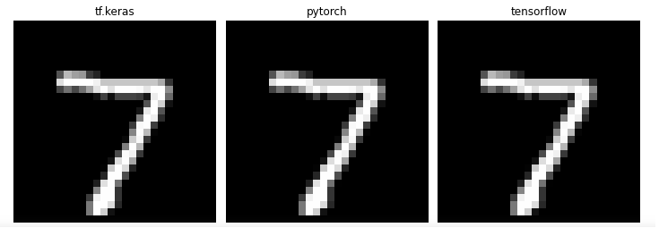
Let's take first image from the test split for each dataset and compare their visualizations.
And as we can see from the output, all images exactly the same. To check other samples just change the identifier for each sample and repeat the procedure. But we can already say that we deal with the same datasets despite they were obtained in different ways.

And now we are starting to build our neural networks!
🇰 Keras
We will keep our order and start from keras. We need to export 5 types of layers. All of them will be used in our implementation. One more thing before we start - we will build the same architecture using two different coding styles. There is no any changes in the logic just two different approaches to write code in keras framework.
First one - we will use Sequential model and will add each layer to the list of layers as you can see below. For each of the convolutional layers we are using relu activation function. For the output layer we take softmax function.
As a result we have next ready for training neural network.
Model: "sequential"
_________________________________________________________________
 Layer (type)                Output Shape              Param #
=================================================================
 conv2d (Conv2D)             (None, 26, 26, 32)        320

 max_pooling2d (MaxPooling2D  (None, 13, 13, 32)       0
 )

 conv2d_1 (Conv2D)           (None, 11, 11, 64)        18496

 max_pooling2d_1 (MaxPooling  (None, 5, 5, 64)         0
 2D)

 flatten (Flatten)           (None, 1600)              0

 dropout (Dropout)           (None, 1600)              0

 dense (Dense)               (None, 10)                16010

=================================================================
Total params: 34,826
Trainable params: 34,826
Non-trainable params: 0
_________________________________________________________________
Now we are building the same model but using signal propagation style. The main difference from previous notation is that we need to specify here the output from the layer as an input for the next layer.
As we can see the number of parameters exactly the same so both models are equal.
Model: "model"
_________________________________________________________________
 Layer (type)                Output Shape              Param #
=================================================================
 input_2 (InputLayer)        [(None, 28, 28, 1)]       0

 conv2d_2 (Conv2D)           (None, 26, 26, 32)        320

 max_pooling2d_2 (MaxPooling  (None, 13, 13, 32)       0
 2D)

 conv2d_3 (Conv2D)           (None, 11, 11, 64)        18496

 max_pooling2d_3 (MaxPooling  (None, 5, 5, 64)         0
 2D)

 flatten_1 (Flatten)         (None, 1600)              0

 dropout_1 (Dropout)         (None, 1600)              0

 dense_1 (Dense)             (None, 10)                16010

=================================================================
Total params: 34,826
Trainable params: 34,826
Non-trainable params: 0
_________________________________________________________________
Finally we are defining optimizer and loss function, compiling our model and starting to train it. As an optimizer we will use Adam with default parameters except learning rate. As a loss function we use categorical crossentropy. Also we take accuracy as a target metric.
Also one important moment here - we don't have prepared in advance validation set. This can be solved specifying validation_split parameter inside fit function. This means that we will use 10% of our training set as validation split.
Your output will be similar to this:
Epoch 1/5
422/422 [==============================] - 25s 58ms/step - loss: 0.3646 - accuracy: 0.8875 - val_loss: 0.0875 - val_accuracy: 0.9765
Epoch 2/5
422/422 [==============================] - 25s 58ms/step - loss: 0.1120 - accuracy: 0.9663 - val_loss: 0.0620 - val_accuracy: 0.9837
Epoch 3/5
422/422 [==============================] - 25s 58ms/step - loss: 0.0844 - accuracy: 0.9740 - val_loss: 0.0471 - val_accuracy: 0.9880
Epoch 4/5
422/422 [==============================] - 22s 53ms/step - loss: 0.0702 - accuracy: 0.9783 - val_loss: 0.0456 - val_accuracy: 0.9863
Epoch 5/5
422/422 [==============================] - 23s 55ms/step - loss: 0.0627 - accuracy: 0.9813 - val_loss: 0.0429 - val_accuracy: 0.9890
Let's check our scores on the test set after model training finished. Also we will store the result into the dictionary for final analysis.
Scores:
Test loss: 0.038
Test accuracy: 0.988
🇹 Torch
Time to build torch model.
We will define CNN class that represents exactly the same architecture of neural network.
Let's build it and specify loss function and optimizer. We will use the same categorical crossentropy and Adam as we already did.
As we can see we have the same architecture as constructed with keras.
CNN(
  (conv1): Conv2d(1, 32, kernel_size=(3, 3), stride=(1, 1))
  (conv2): Conv2d(32, 64, kernel_size=(3, 3), stride=(1, 1))
  (activation): ReLU()
  (pool): MaxPool2d(kernel_size=2, stride=2, padding=0, dilation=1, ceil_mode=False)
  (drop): Dropout(p=0.5, inplace=False)
  (out): Linear(in_features=1600, out_features=10, bias=True)
)
In torch we need to build custom train function. We need to inform that we are in the train mode (row 2). This is important in several cases. For example in the train mode gradients will be updated on every step. Also dropout is working only during the training.
The output for training:
Epoch [1/5], Step [100/469], Loss: 0.3294
Epoch [1/5], Step [200/469], Loss: 0.1521
Epoch [1/5], Step [300/469], Loss: 0.1407
Epoch [1/5], Step [400/469], Loss: 0.1431
Epoch [2/5], Step [100/469], Loss: 0.0933
Epoch [2/5], Step [200/469], Loss: 0.0959
Epoch [2/5], Step [300/469], Loss: 0.0502
Epoch [2/5], Step [400/469], Loss: 0.1140
Epoch [3/5], Step [100/469], Loss: 0.0835
Epoch [3/5], Step [200/469], Loss: 0.0436
Epoch [3/5], Step [300/469], Loss: 0.1225
Epoch [3/5], Step [400/469], Loss: 0.0358
Epoch [4/5], Step [100/469], Loss: 0.0959
Epoch [4/5], Step [200/469], Loss: 0.0584
Epoch [4/5], Step [300/469], Loss: 0.0507
Epoch [4/5], Step [400/469], Loss: 0.1131
Epoch [5/5], Step [100/469], Loss: 0.0215
Epoch [5/5], Step [200/469], Loss: 0.0163
Epoch [5/5], Step [300/469], Loss: 0.0564
Epoch [5/5], Step [400/469], Loss: 0.0454
As well as for training we need to build evaluation function. Let's also check the score ans save it for the final analysis. We can see that here we change our mode (row 2). It is already changed to evaluation. And after scores calculated we add it to the scores dictionary.
Score:
Test accuracy: 0.988🇹 🇫 TensorFlow
Time to check tensorflow models. In this tutorial we will go through two different approaches.
First one approach - using native tensorflow functions. Let's define layers that will be used inside our neural network. We need to have convolutional, maxpolling and dense layers.
Now we will build a skeleton of our network. We will construct here weight matrix. In the first row we define weight initializer. There is no strict rules how to define it, you can select any other initializer. For each of the layers we also specifying their parameter: for convolutional layers 4 values - size of kernel (2 values), number of input channels and number of output channels. For the dense layer we just need to specify input and output sizes. Maxpooling layer doesn't require any definition because it is just resizing operation.
After we complete skeleton construction we need to define our model. Only one thing here that we should care is to use dropout only in the train mode. For this purpose just add parameter training that will inform model about the training/validation mode.
The same as for all other models we use here categorical crossentropy as a loss function and Adam as optimizer.
Next step is to define our training function. Here we will train our model using training steps. Every time when we call this function the loss will be calculated. Based on this information we will calculate gradients and apply it to optimizer.
The output for training:
Epoch [1/5]
Loss: 2.3161
Loss: 0.1552
Loss: 0.1337
Epoch [2/5]
Loss: 0.1660
Loss: 0.0848
Loss: 0.1191
Epoch [3/5]
Loss: 0.1224
Loss: 0.0505
Loss: 0.1078
Epoch [4/5]
Loss: 0.0651
Loss: 0.0687
Loss: 0.1066
Epoch [5/5]
Loss: 0.0613
Loss: 0.0825
Loss: 0.0794
Final step here is to define evaluation function and add our scores to the scores dictionary.
Score:
Test accuracy: 0.987🇹 🇫 TensorFlow version 2
Second version of the tensorflow implementation is some hybrid between tensorflow and keras. We will use keras layers inside the neural network but will build training process using tensorflow native tools.
Now we are defining the same model but using some other notation. But as you can see the structure is really similar to one that we already did with tf.keras.
Loss function and optimizer still the same.
Training step is really similar to the first version of tensorflow implementation.
Let's train our model.
The output for training:
Epoch [1/5], Loss: 0.3556
Epoch [2/5], Loss: 0.1155
Epoch [3/5], Loss: 0.0862
Epoch [4/5], Loss: 0.0716
Epoch [5/5], Loss: 0.0632
And the last step - as usual to evaluate our model. Again we need to write some custom function for this purpose. Function looks really similar to the previous version.
Score:
Test accuracy: 0.986🏁 Results
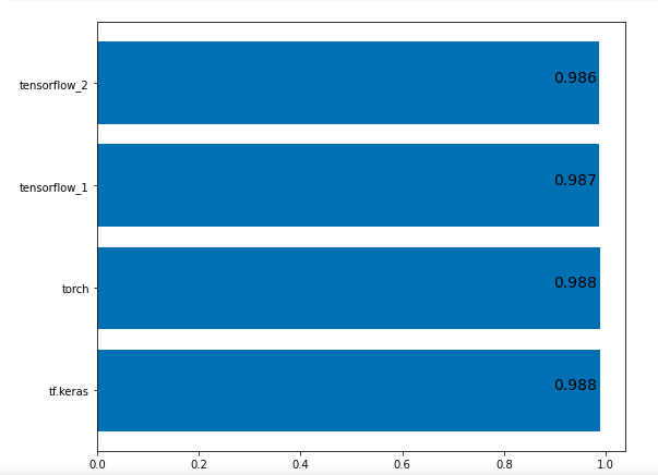
As a final step of our coding exercise - we need to visualize all scores that we collected during the experiments. Let's use bar chart from matplotlib for this purpose.
As we can see all scores almost equal so we can summarize that quality of your model is framework independent and shouldn't be a reason for selection any library.

Thanks for reading this tutorial! Hope it was really useful for you and you find some interesting hints here. Please write in comments, what approach do you prefer and see you on the next papers and tutorials!


Comments